A tasty 3D homogeneous isotropic turbulence dataset

Published 2025-08-04

Introduction

I recently came across a 3D homogeneous isotropic turbulence (HIT) dataset from RWTH Aachen. I like this dataset because:

it was easy to access
it’s well-documented
there’s a reasonable amount of training data
there are pre-computed inputs/targets for superresolution

So I’m putting together this blog post to show how to access the data, and what it looks like. This document from Ludovico Nista et al. contains more details; the point of this post is to be a friendly introduction to this dataset.

Basic overview

There are two flows in the dataset:

forced homogeneous isotropic turbulence
decaying homogeneous isotropic turbulence

The following formats are available:

original DNS velocity fields on a $512^3$ mesh
curated dataset for superresolution, with corresponding pairs of low res (filters) and high res $64^3$ subboxes of the original domain.

Accessing the dataset

You need AWS CLI to access the dataset. Here’s how I installed AWS CLI on Linux, based on the install instructions.

curl "https://awscli.amazonaws.com/awscli-exe-linux-x86_64.zip" -o "awscliv2.zip"
unzip awscliv2.zip
sudo ./aws/install

There are four datasets:

forced HIT, original
forced HIT, curated
decaying HIT, original
decaying HIT, curated

Let’s set up the profiles for both curated datasets.

Forced 3D HIT profile

Run:

aws configure --profile subboxes-forced

When prompted for the AWS Access Key ID, enter

read_a9ba76c4-2bd9-4f96-9758-0999a0fe87a4

When prompted for the secret access key, enter

CvTGQJ5pbCgtQJ6zbbP6TBSYBtqM1lCw

Leave default region name and default output format as empty.

Decaying 3D HIT profile

Run:

aws configure --profile subboxes-decaying

When prompted for the AWS Access Key ID, enter

read_a4d61e08-ba64-4bc8-b790-d6cf5ca6ebd9

When prompted for the secret access key, enter

jsLa4DjRKn7YkJmItx4qJvJR7I7gB3ks

Leave default region name and default output format as empty.

Looking around the dataset

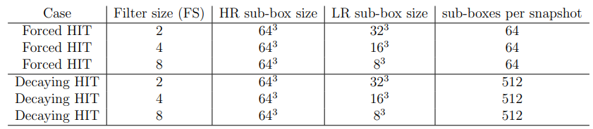
As of right now (August 1 2025), the structure is a little inconsistent, but we get the general vibe. The key to understanding this structure, and what’s available, is this table from the author’s document:

Available data

Forced HIT dataset

I ran this to see the folder structure, without the .h5 data files:

aws s3 ls s3://a9ba76c4-2bd9-4f96-9758-0999a0fe87a4/   --endpoint-url=https://coscine-s3-01.s3.fds.rwth-aachen.de:9021   --profile subboxes-forced --recursive |   awk '{print $4}' | sed 's|^|./|' | tree --fromfile -I "*.h5"

And we can see:

.
└── .
    ├── Delta2
    │   ├── Boxes32
    │   │   ├── CombineSnapshots.py
    │   │   ├── DNS
    │   │   │   ├── stage_reduced_1
    │   │   │   ├── TEST
    │   │   │   └── VALID
    │   │   └── LES
    │   │       ├── stage_reduced_1
    │   │       ├── TEST
    │   │       └── VALID
    │   ├── Boxes_Gaussian32
    │   │   ├── CombineSnapshots.py
    │   │   ├── DNS
    │   │   │   ├── stage_reduced_1
    │   │   │   ├── TEST
    │   │   │   └── VALID
    │   │   └── LES
    │   │       ├── stage_reduced_1
    │   │       ├── TEST
    │   │       └── VALID
    │   ├── Boxes_Spectral32
    │   │   ├── CombineSnapshots.py
    │   │   ├── DNS
    │   │   │   ├── stage_reduced_1
    │   │   │   ├── stage_reduced_2
    │   │   │   └── VALID
    │   │   └── LES
    │   │       ├── stage_reduced_1
    │   │       ├── stage_reduced_2
    │   │       └── VALID
    │   └── MakeBoxes_HIT.py
    ├── Delta4
    │   ├── Box
    │   │   ├── Boxes16
    │   │   │   ├── CombineSnapshots.py
    │   │   │   ├── DNS
    │   │   │   │   ├── stage_reduced_1
    │   │   │   │   ├── TEST
    │   │   │   │   └── VALID
    │   │   │   └── LES
    │   │   │       ├── stage_reduced_1
    │   │   │       ├── TEST
    │   │   │       └── VALID
    │   │   └── MakeBoxes_HIT.py
    │   ├── Gaussian
    │   │   ├── CombineSnapshots.py
    │   │   ├── DNS
    │   │   │   ├── stage_1
    │   │   │   ├── stage_reduced_1
    │   │   │   ├── stage_reduced_2
    │   │   │   ├── stage_reduced_3
    │   │   │   ├── TEST
    │   │   │   └── VALID
    │   │   └── LES
    │   │       ├── stage_1
    │   │       ├── stage_reduced_1
    │   │       ├── stage_reduced_2
    │   │       ├── stage_reduced_3
    │   │       ├── TEST
    │   │       └── VALID
    │   └── Spectral
    │       └── Boxes16
    │           ├── CombineSnapshots.py
    │           ├── DNS
    │           │   ├── stage_reduced_1
    │           │   ├── TEST
    │           │   └── VALID
    │           └── LES
    │               ├── stage_reduced_1
    │               ├── TEST
    │               └── VALID
    └── Delta8
        ├── Boxes8
        │   ├── CombineSnapshots.py
        │   ├── DNS
        │   │   ├── stage_reduced_1
        │   │   ├── TEST
        │   │   └── VALID
        │   └── LES
        │       ├── stage_reduced_1
        │       ├── TEST
        │       └── VALID
        └── MakeBoxes_HIT.py

Decaying HIT dataset

Here’s the equivalent command for the decaying HIT dataset:

aws s3 ls s3://a4d61e08-ba64-4bc8-b790-d6cf5ca6ebd9/   --endpoint-url=https://coscine-s3-01.s3.fds.rwth-aachen.de:9021   --profile subboxes-decaying --recursive |   awk '{print $4}' | sed 's|^|./|' | tree --fromfile -I "*.h5"

.
└── .
    └── Delta8
        ├── Box
        │   ├── Boxes8
        │   │   ├── CombineSnapshots.py
        │   │   ├── DNS
        │   │   │   ├── stage_reduced_1
        │   │   │   └── VALID
        │   │   └── LES
        │   │       ├── stage_reduced_1
        │   │       └── VALID
        │   └── MakeBoxes_HIT.py
        ├── Gaussian
        │   ├── Boxes8
        │   │   ├── CombineSnapshots.py
        │   │   ├── DNS
        │   │   │   ├── stage_reduced_1
        │   │   │   └── VALID
        │   │   └── LES
        │   │       ├── stage_reduced_1
        │   │       └── VALID
        │   └── MakeBoxes_HIT.py
        └── Spectral
            ├── Boxes8
            │   ├── CombineSnapshots.py
            │   ├── DNS
            │   │   ├── stage_reduced_1
            │   │   └── VALID
            │   └── LES
            │       ├── stage_reduced_1
            │       └── VALID
            └── MakeBoxes_HIT.py

Downloading the dataset

I’m going to download the dataset without the pre-combined time series files as I’d like to be able to work with the raw data myself, and merge it how I like.

Here are some useful commands:

Download the entire dataset

Forced HIT (300 GB download)

aws s3 sync s3://a9ba76c4-2bd9-4f96-9758-0999a0fe87a4/ ./forced_hit_complete/ --endpoint-url=https://coscine-s3-01.s3.fds.rwth-aachen.de:9021 --profile subboxes-forced --exclude "stage_reduced_*/*"

Decaying HIT (100 GB Download)

aws s3 sync s3://a4d61e08-ba64-4bc8-b790-d6cf5ca6ebd9/ ./decaying_hit_complete/ --endpoint-url=https://coscine-s3-01.s3.fds.rwth-aachen.de:9021 --profile subboxes-decaying --exclude "stage_reduced_*/*"

If you don’t want to download the whole dataset at once, you can access the directories based on the structure I gave above. For example, something like

aws s3 sync s3://a4d61e08-ba64-4bc8-b790-d6cf5ca6ebd9/path/to/dataset/directory /path/to/local/storage --endpoint-url=https://coscine-s3-01.s3.fds.rwth-aachen.de:9021 --profile subboxes-decaying

Visualizing the dataset

All code for visualization is availalble in the git repo for this blog post. I have a script which takes the original dataset format ($N$ boxes per $T$ timesteps) and extracts an individual numpy array for each box for each timestep. It’s appropriately called extract_individual_numpy_arrays.py in my repo.

I’m going to visualize the DNS data that comes with the box filtered data for the FS8 task.

Velocity magnitude

Let’s look at the velocity magnitude for all 64 boxes from the forced HIT DNS dataset.

We can see that generally, the velocity magnitude remains the same throughout the dataset. It is, in fact, forced HIT. That’s kind of the point!

Similarly, here are all 32 boxes from the decaying HIT dataset:

The velocity magnitude decays, because this is a decaying HIT dataset.

$Q$-criterion

The $Q$-criterion sounds like some some sort of conspiracy theory, but it’s much more boring than that. It’s used to visualize vortex structures in a turbulent flow. It’s calculated by

\[Q = \frac{1}{2}\left(||R||^2-||S||^2 \right) \ ,\]

where $||\cdot||^2$ is the Frobenius norm of a tensor, $R$ is the rotation rate tensor, and $S$ is the strain rate tensor. To take the Frobenius norm, you just individually square each element, and then sum them up (remember, code is provided with this post so you can see exactly how I do it). More information about the $Q$-criterion can be found in these references:

https://www.cambridge.org/core/journals/journal-of-fluid-mechanics/article/on-the-relationships-between-local-vortex-identification-schemes/E1DE98BE2DACF2A1724F62322C7FAFEB
https://pubs.aip.org/aip/pof/article/31/12/121701/957670/Comparison-between-the-Q-criterion-and-Rortex-in

$Q$-criterion measures excess strain to rotation rate. When $Q>0$, it indicates regions where vorticity dominantes over strain (because the rotation rate tensor $R$ has a higher Frobenius norm than the strain rate tensor $S$).

Here’s an animation of isosurface of $Q = 0.05$, for a single box of the forced turbulence dataset. It’s coloured by velocity magnitude. This lets us see the vortices, coloured by the speed at which the vortex structure is moving.

A couple of notes

The dataset is dimensional. These velocities are in units of m/s. Details on the mesh spacing can be found in the dataset documentation. This is cool! Often, DNS data is non-dimensionalized in a way that hurts my smooth brain.
The subboxes for the different tasks are different. For example, while the target boxes for the FS4 Box filtered data correspond to the input boxes for this specific task, they are different than the target boxes from the FS4 Spectral filtered data.

Computing the turbulent kinetic energy spectrum

In this blog post, I document in a high level of detail how to compute the turbulent kinetic energy spectrum for this flow.