The nuts and bolts of the PISO algorithm; visualizing discretization matrices in OpenFOAM
Published 2025-04-23
The github repo for this blog post is here. It contains
- OpenFOAM case setup for the lid driven cavity problem
- The
verbosePisoFoamsolver, which is a modified version ofpisoFoamthat prints out the discretization matrix. - A Python notebook to visualize the discretization matrix.
Introduction
Segregated pressure velocity coupling solvers for the Navier-Stokes equations. Sound familiar? Well, these algorithms were used to design the last car you were in, and the last plane you were in.
For an incompressible, viscous fluid, the Navier-Stokes equations govern the relationship between two variables: pressure $p$, and velocity $\mathbf{U}$. In an incompressible flow, the challenging part of a CFD algorithm is pressure-velocity coupling. We don’t have an “equation of state” (a separate equation for pressure). All we have are two equations: conservation of mass and conservation of momentum. We simultaneously solve this system of equations. Unfortunately, these equations are quite difficult to solve simultaneously.
Equations
The main equation is the momentum equation:
\[\frac{\partial \mathbf{U}}{\partial t} + \nabla \cdot (\mathbf{U} \mathbf{U}) = -\nabla p + \nu \nabla^2 \mathbf{U}\](here, $p$ is the kinematic pressure).
The continuity equation is conservation of mass for an incompressible fluid: $dm/dt = 0$. Since our fluid is incompressible ($\rho$ is constant), this equation is equivalent to a “conservation of volume”: $d(\rho V)/dt = 0 \rightarrow dV/dt = 0$.
\[\nabla \cdot \mathbf{U} = 0\]For more info - check out my blog post on the Navier-Stokes equations.
Discretization
Let’s speedrun through how these two equations are actually solved simultaneously in a CFD algorithm. We discretize these equations on a mesh, using a set of discretization schemes (e.g., upwind, central difference). Often, different terms in the momentum equation are discretized using different schemes. This isn’t important - at the end of the day, we end up with a system of linear equations.
\[\frac{\partial \mathbf{U}}{\partial t} + \nabla \cdot (\mathbf{U} \mathbf{U}) = - \nabla p + \nu \nabla^2 \mathbf{U}\]Using our discretization schemes, this equation is simply written as:
\[M \mathbf{U} = -\nabla p\]The exact schemes used in our discretization of $\mathbf{U}$ are crammed together into one big matrix $M$ of coefficients. These coefficients ($M$) are known. AKA, they are not unknowns. We know $M$. It’s a matrix full of numbers that we know. Remember: our only two unknowns throughout this are are $p$ and $\mathbf{U}$.
Let’s set up a simple lid driven cavity problem on a 3x3 mesh so that we can look at the discretization matrix $M$. All
Let’s look at our matrix $M$ (remember, it’s just matrix full of numbers) for a 3x3 mesh. Let’s visualize it using colours. The darker the colour, the larger the number. Let’s visualize the discretization matrix $M$ in OpenFOAM. The code to do this is attached to this blog post. An important thing to note is that diagonal dominance of this matrix is very important. Stable algorithms tend to have higher diagonal dominance. What’s diagonal dominance? Big number on matrix diagonal, smaller numbers on off-diagonal.
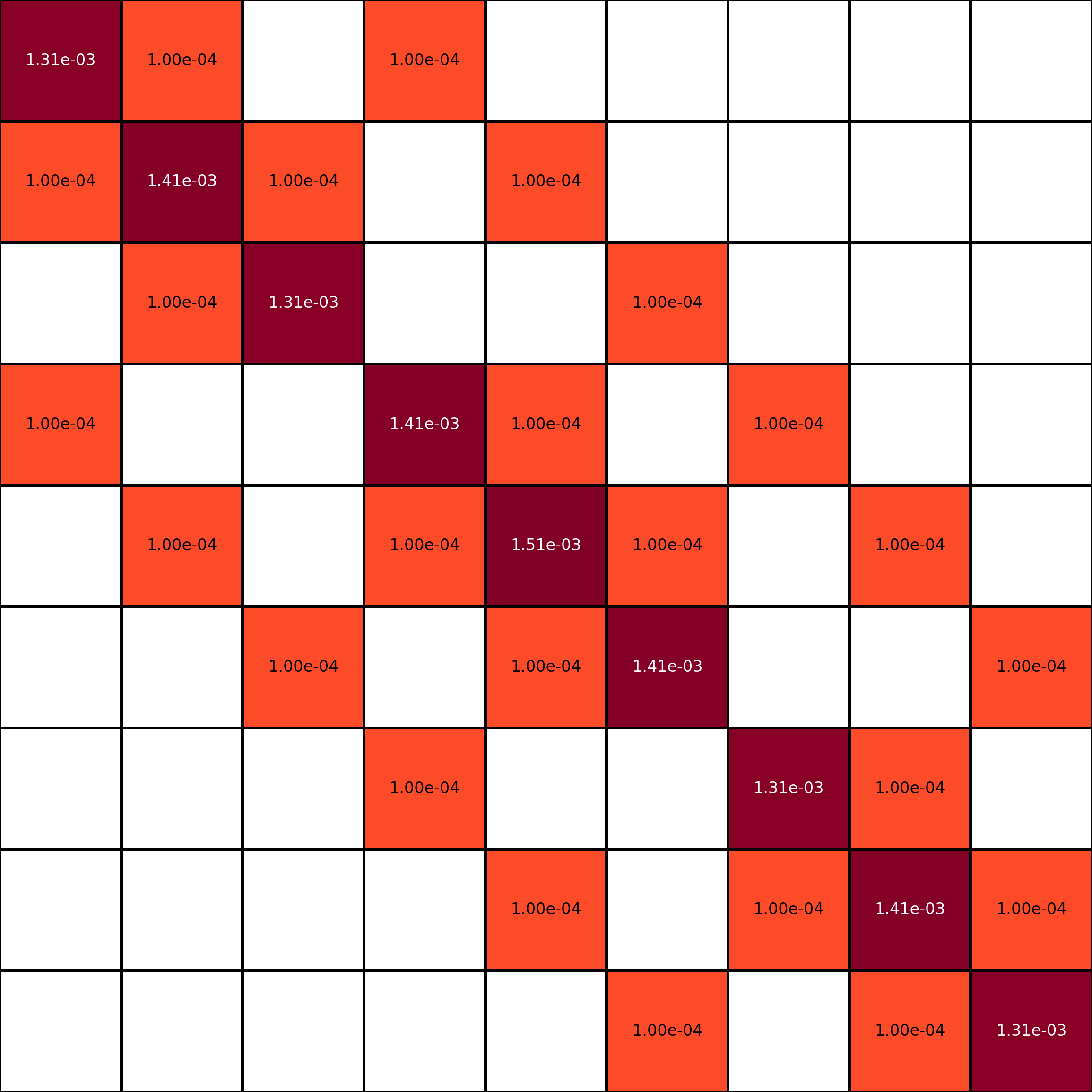
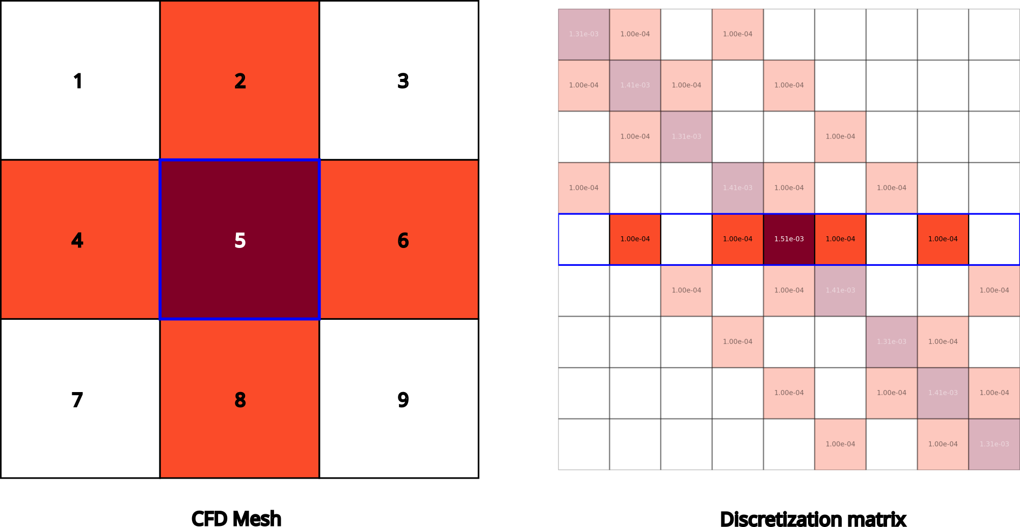
Each row of $M$ corresponds to conservation of momentum for a single cell in the mesh. There are $N$ cells in the mesh, and therefore $M \in \mathbb{R}^{N \times N}$. The diagonal elements are the coefficients for the velocity of the cell itself in the “discretized momentum equation” (i.e., the momentum equation after we substituted in our discretization schemes). The off-diagonal elements are the coefficients for the velocity of all the other cells in the mesh. Conservation of momentum for a given cell usually just considers the neighbouring cells (it’s just a momentum balance over a given cell). For example, the momentum balance for the centre cell in this mesh depends on the velocity of the cell itself, and the velocities of the cells to the north, south, east, and west. Can you identify which row in the matrix corresponds to the momentum balance for the centre cell?

Right, it’s the fifth row! It’s the only one which depends on four other cells (in this specific 3x3 mesh with non-periodic boundary conditions). It’s highlighted in the image below.
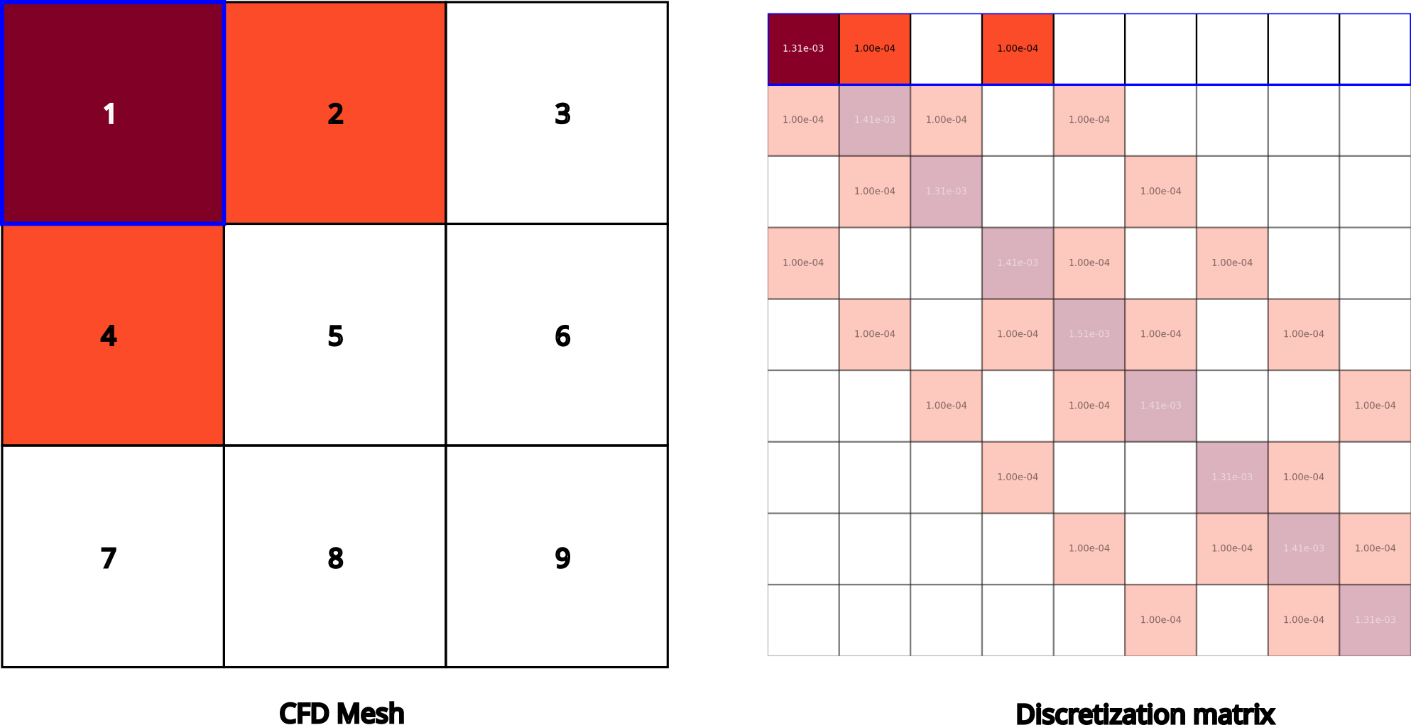
Let’s look at the top left (boundary) cell.
Next, let’s look at a matrix $M$ for a 32x32 mesh (1024x1024 elements in the matrix).
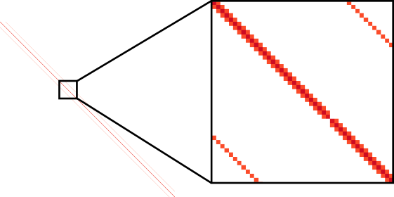

Wow, that’s a big matrix! And this is only a mesh with 1000 cells. Typical industrial simulations have 10’s of millions of cells, or even a billion cells. Do you know how much memory it takes to store a billion X billion matrix? About 8,000 petabytes. This single simulation could use 15% of the available memory on the entire planet Earth. Luckily, we can exploit the sparse nature of $M$ to store it in memory, and solve it using iterative methods, which are a lot more efficient than direct methods. In the case of the above video (billion cell mesh), that can be run on a handful of GPUs.
Remark.
$M$ is:
- mostly zeros (aka sparse)
- block-banded
PISO algorithm
The original reference for the PISO algorithm is from 1986 by Issa et al.. Despite being almost 40 years old at the time of this post, it’s still going strong!
Let’s make the following decomposition:
\[M\mathbf{U} = A\mathbf{U} - H\]Where $A$ is the diagonal part of $M$.
Remark.
$A^{-1}$ is easily computed. Since $A$ a diagonal matrix (it’s the diagonal of $M$), $A^{-1}$ is also a diagonal matrix with elements $1/A_{ij}$ on the diagonal. We’re just doing 1/(each diagonal element of $A$).
Remark.
$M \neq A - H$. The definition of $H$ incorporates $\mathbf{U}$ itself! $A$ is independent of $\mathbf{U}$, but $H$ is not. A given $H$ comes with a given $\mathbf{U}$. When $\mathbf{U}$ updates, we need to update $H$.
This decomposition of $M$ leads to two equations:
- $\mathbf{U} = A^{-1}H - A^{-1}\nabla p$.
- $\nabla \cdot \left(A^{-1}\nabla p\right) = \nabla \cdot \left(A^{-1}H\right)$.
To get 1., we set $A\mathbf{U} - H = -\nabla p$, then multiply by $A^{-1}$ (remember $A^{-1}$ is very easy to compute). To get 2, we use the fact that $\nabla \cdot \mathbf{U} = 0$ (i.e., we just take the divergence of 1, set equal to zero, and rearrange). More details on this can be found in the excellent Fluid Mechanics 101 Video on Youtube. I can’t recommend this Youtube channel enough.
OK, so we have broken our coupled system of 2 equations into 4 equations now:
- $M\mathbf{U} = -\nabla p$ AKA MOMENTUM PREDICTOR. It calculates velocity field $\mathbf{U}$ from pressure field $p$.
- $H = A\mathbf{U} - M\mathbf{U}$ AKA H UPDATER. It calculates $H$ from velocity field $\mathbf{U}$.
- $\nabla \cdot \left(A^{-1}\nabla p\right) = \nabla \cdot \left(A^{-1}H\right)$ AKA PRESSURE CORRECTOR. It calculates pressure field $p$ from $H$.
- $U = A^{-1}H - A^{-1}\nabla p$ AKA VELOCITY UPDATER. It calculates velocity field $\mathbf{U}$ from $H$ and $p$.
A typical PISO loop is: 1->2->3->4->2->3->4. In other words, that’s a momentum corrector followed by two inner loops.
OpenFOAM’s clean implementation of the PISO algorithm is given below.
Info<< "\nStarting time loop\n" << endl;

while (runTime.loop())
{
     Info<< "Time = " << runTime.timeName() << nl << endl;

     #include "CourantNo.H"

     // Update settings from the control dictionary
     piso.read();

     // Pressure-velocity PISO corrector
     {
          #include "UEqn.H"

          // --- PISO loop
          while (piso.correct())
          {
               #include "pEqn.H"
          }
     }

     laminarTransport.correct();
     turbulence->correct();

     runTime.write();

     runTime.printExecutionTime(Info);
}

Info<< "End\n" << endl;